Parallelization using Dask

🧊 Installation

!pip install "dask[complete]"

import dask

dask.__version__

'2023.5.0'

import dask.array as da
import dask.bag as db
import dask.dataframe as dd
import numpy as np
import pandas as pd

🪐 Basic Concepts of Dask

On a high-level, you can think of Dask as a wrapper that extends the capabilities of traditional tools like pandas, NumPy, and Spark to handle larger-than-memory datasets.

When faced with large objects like larger-than-memory arrays (vectors) or matrices (dataframes), Dask breaks them up into chunks, also called partitions.

For example, consider the array of 12 random numbers in both NumPy and Dask:

narr = np.random.rand(12)

narr

array([0.44236558, 0.00504448, 0.87087911, 0.468925  , 0.37513511,
       0.22607761, 0.83035297, 0.07772372, 0.61587933, 0.82861156,
       0.66214299, 0.90979423])

darr = da.from_array(narr, chunks=3)
darr

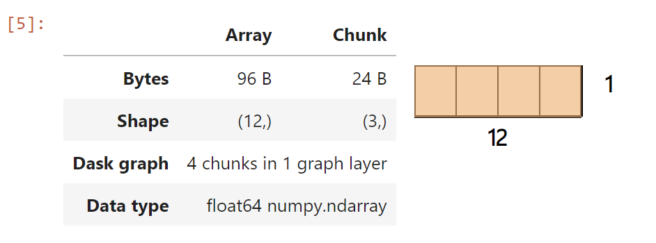
The image above shows that the Dask array contains four chunks as we set chunks to 3. Under the hood, each chunk is a NumPy array in itself.

To fully appreciate the benefits of Dask, we need a large dataset, preferably over 1 GB in size. Consider the autogenerated data from the script below:

import string

# Set the desired number of rows and columns
num_rows = 5_000_000
num_cols = 10
chunk_size = 100_000

# Define an empty DataFrame to store the chunks
df_chunks = pd.DataFrame()

# Generate and write the dataset in chunks
for i in range(0, num_rows, chunk_size):
    # Generate random numeric data
    numeric_data = np.random.rand(chunk_size, num_cols)

    # Generate random categorical data
    letters = list(string.ascii_uppercase)
    categorical_data = np.random.choice(letters, (chunk_size, num_cols))

    # Combine numeric and categorical data into a Pandas DataFrame
    df_chunk = pd.DataFrame(np.concatenate([numeric_data, categorical_data], axis=1))

    # Set column names for better understanding
    column_names = [f'Numeric_{i}' for i in range(num_cols)] + [f'Categorical_{i}' for i in range(num_cols)]
    df_chunk.columns = column_names

    # Append the current chunk to the DataFrame holding all chunks
    df_chunks = pd.concat([df_chunks, df_chunk], ignore_index=True)

    # Write the DataFrame chunk to a CSV file incrementally
    if (i + chunk_size) >= num_rows or (i // chunk_size) % 10 == 0:
        df_chunks.to_csv('large_dataset.csv', index=False, mode='a', header=(i == 0))
        df_chunks = pd.DataFrame()

dask_df = dd.read_csv("large_dataset.csv")

dask_df.head()

Even though the file is large, you will notice that the result is fetched almost instantaneously. For even larger files, you can specify the blocksize parameter, which determines the number of bytes to break up the file into.

Similar to how Dask Arrays contain chunks of small NumPy arrays, Dask is designed to handle multiple small Pandas DataFrames arranged along the row index.

✨ Selecting columns and element-wise operations

In this example, we're doing some pretty straightforward column operations on our Dask DataFrame, called dask_df. We're adding the values from the column Numeric_0 to the result of multiplying the values from Numeric_9 and Numeric_3. We store the outcome in a variable named result.

result = (
   dask_df["Numeric_0"] + dask_df["Numeric_9"] * dask_df["Numeric_3"]
)

result.compute().head()

As we’ve mentioned, Dask is a bit different from traditional computing tools in that it doesn't immediately execute these operations. Instead, it creates a kind of 'plan' called a task graph to carry out these operations later on. This approach allows Dask to optimize the computations and parallelize them when needed. The compute() function triggers Dask to finally perform these computations, and head() just shows us the first few rows of the result.

⚡️ Conditional filtering

Now, let's look at how Dask can filter data. We're selecting rows from our DataFrame where the value in the "Categorical_5" column is "A".

This filtering process is similar to how you'd do it in pandas, but with a twist - Dask does this operation lazily. It prepares the task graph for this operation but waits to execute it until we call compute(). When we run head(), we get to see the first few rows of our filtered DataFrame.

dask_df[dask_df["Categorical_5"] == "A"].compute().head()

✨ Common summary statistics

Next, we're going to generate some common summary statistics using Dask's describe() function.

It gives us a handful of descriptive statistics for our DataFrame, including the mean, standard deviation, minimum, maximum, and so on. As with our previous examples, Dask prepares the task graph for this operation when we call describe(), but it waits to execute it until we call compute().

dask_df.describe().compute()

dask_df["Categorical_3"].value_counts().compute().head()

We also use value_counts() to count the number of occurrences of each unique value in the "Categorical_3" column. We trigger the operation with compute(), and head() shows us the most common values.

✨ Groupby

Finally, let's use the groupby() function to group our data based on values in the "Categorical_8" column. Then we select the "Numeric_7" column and calculate the mean for each group.

This is similar to how you might use ‘groupby()’ in pandas, but as you might have guessed, Dask does this lazily. We trigger the operation with compute(), and head() displays the average of the "Numeric_7" column for the first few groups.

dask_df.groupby("Categorical_8")["Numeric_7"].mean().compute().head()

⚡️ Lazy evaluation

Now, let’s explore the use of the compute function at the end of each code block.

Dask evaluates code blocks in lazy mode compared to Pandas’ eager mode, which returns results immediately.

To draw a parallel in cooking, lazy evaluation is like preparing ingredients and chopping vegetables in advance but only combining them to cook when needed. The compute function serves that purpose.

In contrast, eager evaluation is like throwing ingredients into the fire to cook as soon as they are ready. This approach ensures everything is ready to serve at once.

Lazy evaluation is key to Dask’s excellent performance as it provides:

1. Reduced computation. Expressions are evaluated only when needed (when compute is called), avoiding unnecessary intermediate results that may not be used in the final result.
2. Optimal resource allocation. Lazy evaluation avoids allocating memory or processing power to intermediate results that may not be required.
3. Support for large datasets. This method processes data elements on-the-fly or in smaller chunks, enabling efficient utilization of memory resources.

When the results of compute are returned, they are given as Pandas Series/DataFrames or NumPy arrays instead of native Dask DataFrames.

type(dask_df)

dask.dataframe.core.DataFrame

type(
   dask_df[["Numeric_5", "Numeric_6", "Numeric_7"]].mean().compute()
)

pandas.core.series.Series

The reason for this is that most data manipulation operations return only a subset of the original dataframe, taking up much smaller space. So, there won’t be any need to use parallelism of Dask, and you continue the rest of your workflow either in pandas or NumPy.

🪐 Dask Bags and Dask Delayed for Unstructured Data

Dask Bags and Dask Delayed are two components of the Dask library that provide powerful tools for working with unstructured or semi-structured data and enabling lazy evaluation.

While in the past, tabular data was the most common, today’s datasets often involve unstructured files such as images, text files, videos, and audio. Dask Bags provides the functionality and API to handle such unstructured files in a parallel and scalable manner.

For example, let’s consider a simple illustration:

# Create a Dask Bag from a list of strings
b = db.from_sequence(["apple", "banana", "orange", "grape", "kiwi"])

# Filter the strings that start with the letter 'a'
filtered_strings = b.filter(lambda x: x.startswith("a"))

# Map a function to convert each string to uppercase
uppercase_strings = filtered_strings.map(lambda x: x.upper())

# Compute the result as a list
result = uppercase_strings.compute()

print(result)

['APPLE']

In this example, we create a Dask Bag b from a list of strings. We then apply operations on the Bag to filter the strings that start with the letter 'a' and convert them to uppercase using the filter() and map() functions, respectively. Finally, we compute the result as a list using the compute() method and print the output.

Now imagine that you can perform even more complex operations on billions of similar strings stored in a text file. Without the lazy evaluation and parallelism offered by Dask Bags, you would face significant challenges.

As for Dask Delayed, it provides even more flexibility and introduces lazy evaluation and parallelism to various other scenarios. With Dask Delayed, you can convert any native Python function into a lazy object using the @dask.delayed decorator.

Here is a simple example:

%%time

import time
@dask.delayed
def process_data(x):
   # Simulate some computation
   time.sleep(1)
   return x**2


# Generate a list of inputs
inputs = range(1000)

# Apply the delayed function to each input
results = [process_data(x) for x in inputs]

# Compute the results in parallel
computed_results = dask.compute(*results)

CPU times: user 260 ms, sys: 68.1 ms, total: 328 ms
Wall time: 32.2 s

In this example, we define a function process_data decorated with @dask.delayed. The function simulates some computational work by sleeping for 1 second and then returning the square of the input value.

Without parallelism, performing this computation on 1000 inputs would have taken more than 1000 seconds. However, with Dask Delayed and parallel execution, the computation only took about 42.1 seconds.

This example demonstrates the power of parallelism in reducing computation time by efficiently distributing the workload across multiple cores or workers.

That’s what parallelism is all about. for more information see https://docs.dask.org/en/stable/